How to use Excel's INDEX Function
Returns a value from a range based on the position specified
What does Excel's INDEX function do?
The INDEX function is one of Excel's lookup and reference functions.
In financial modelling we use the INDEX function to return a value from a range based on the position specified. In scenario modelling we can use INDEX to pull the values for the selected scenario.
INDEX is often combined with the MATCH function to to map data from one table into another based on a unique reference.
Here's a simple example
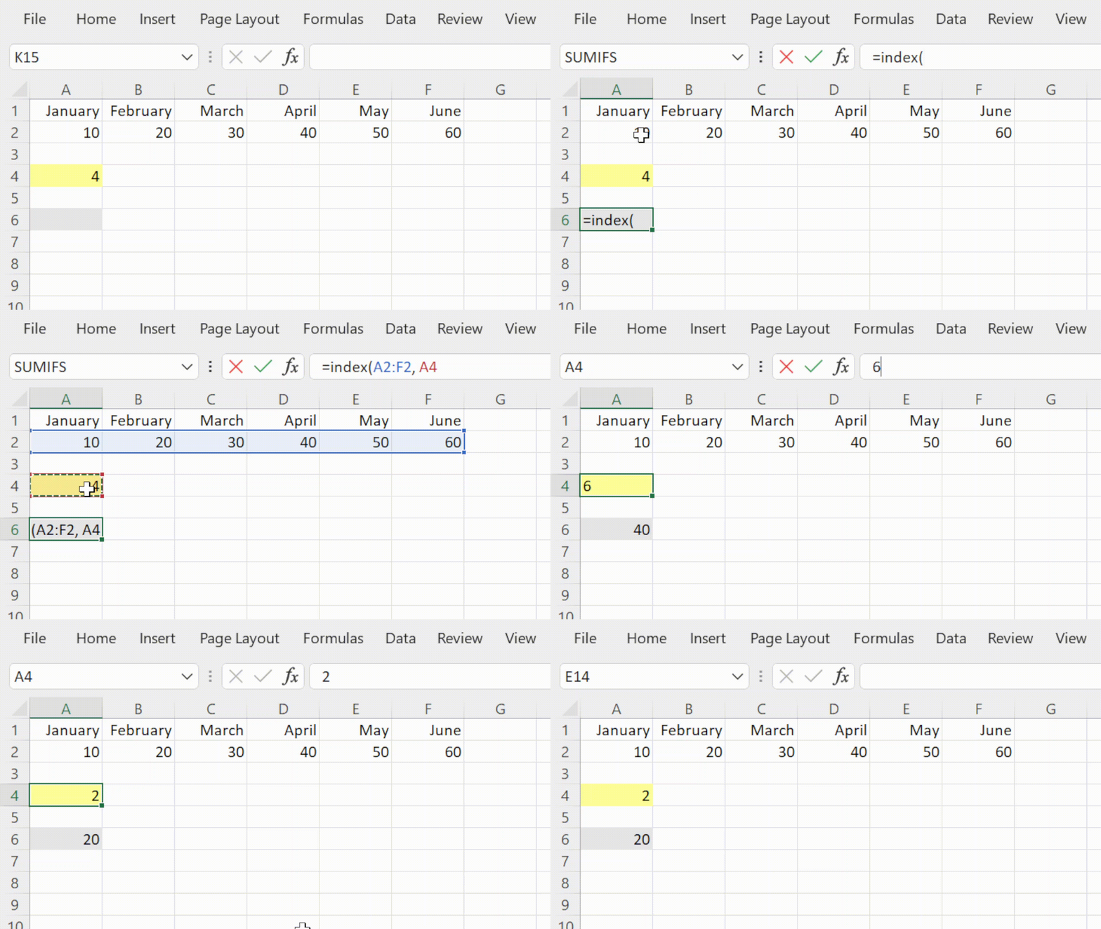
Let's take a look at a simple example of the INDEX function.
We have a set of numbers in the cell range A2 to F2.
We would like to return the forth item in that range.
We would write the formula using INDEX as follows:
=INDEX(A2:F2,4)

What does that mean in plain English?
Return the value in the fourth position in the range A2 to F2.
How do I write a formula using the INDEX function?
=INDEX(array, row number, [column number])
array – The range of cells that you want to analyse.
row number – The number of the row that you want to return a value for. This is the number of the item in a list arranged vertically.
[column number] – The number of the column that you want to return a value for. This is the number of the item in a list arranged horizontally.
What to consider when using the INDEX function in your financial model
- Avoid using full column and row references as this is very inefficient.
- Combine with MATCH for a clear, flexible and efficient lookup formula.
- INDEX MATCH can often be used instead of complex nested IF functions.
- The XLOOKUP function can be used in place of INDEX MATCH
Read more about the INDEX function on the Microsoft support page here.

